- EDITOR’S NOTE: I highly recommend watching videos/demos of these topics
and/or playing around with these algorithms and concepts yourself, the definitions and examples in
text form won’t be enough to fully understand the concept behind these algorithms - they are merely
here to provide a rough blueprint
- try and do the tutorial exerices, solve old exams or use a tool like TUMGAD to automatically generate exercises and corresponding solutions
Complexity
- Time Complexity: relation
between growth of runtime and growth of input
- I: set of instances of an algorithm with different inputs
- T: I \to \N: runtime of an algorithm, usually measured in an actual unit of time (e.g. nanoseconds)
- Space Complexity: relation between used space / memory and growth of input
Different Cases
- I_n: set of instances of size n
- worst case: t(n) =
\max\{T(i) : i \in I_n\}
- pessimistic, but guarantees efficiency
- average case: t(n) =
\frac{1}{|I_n|} \sum_{i \in I_n}T(i) if I_n \in \N, else t(n) = \sum_{i \in I_n} P[i] \cdot
T(i)
- average, but doesn’t necessarily define usual behavior
- best case: t(n) =
\min\{T(i) : i \in I_n\}
- best result possible, but very optimistic
Landau-Notation
- limiting behavior when the argument tends towards a particular
value or infinity
- g \in \mathcal{O}(f(n)) =
\{g(n) \; | \; \exists c > 0 \; \exists n_0 > 0 \; \forall n \geq n_0 : g(n)
\leq c \cdot f(n)\}
- functions that do not grow faster asymptotically than f (upper asymptotic bound)
- g(n) \in \mathcal{O}(f(n)) \equiv g is at most a positive constant multiple of f for all sufficiently large values of n
- g \in \mathcal{o}(f(n)) =
\{g(n) \; | \; \forall C > 0 \; \exists n_0 > 0 \; \forall n \geq n_0 : g(n)
\leq C \cdot f(n)\}
- functions that grow slower than f
- \mathcal{o}(f(n)) \subseteq \mathcal{O}(f(n))
- g \in \Omega(f(n)) = \{g(n)
\; | \; \exists c > 0 \; \exists n_0 > 0 \; \forall n \geq n_0 : g(n) \geq c
\cdot f(n)\}
- functions that do not grow slower asymptotically than f (lower asymptotic bound)
- g \in \omega(f(n)) = \{g(n)
\; | \; \forall C > 0 \; \exists n_0 > 0 \; \forall n \geq n_0 : g(n) \geq C
\cdot f(n)\}
- functions that grow faster than f
- \omega(f(n)) \subseteq \Omega(f(n))
- g \in \Theta(f(n)) =
\mathcal{O}(f(n)) \cap \Omega(f(n))
- functions that have the same growth rate as f
- \Theta(f(n)) \subseteq \mathcal{O}(f(n)) and \Theta(f(n)) \subseteq \Omega(f(n))
- g \in \mathcal{O}(f(n)) =
\{g(n) \; | \; \exists c > 0 \; \exists n_0 > 0 \; \forall n \geq n_0 : g(n)
\leq c \cdot f(n)\}
- (!) \omega(f(n)) \cap o(f(n)) = \emptyset
- (!) f(n) \in o(g(n)) \implies g(n) \in \omega(f(n))
- some use case examples…
- 5n^2-7n \in \mathcal{O}(n^2), but also \mathcal{O}(n^3), \mathcal{O}(n^4)... (also included in “greater” sets, since \mathcal{O} defines the upper bound)
- 5n^2-7n \in \Omega(n^2), but also \Omega(n) (also included in “lesser” sets, since \Omega defines the lower bound)
- 5n^2-7n \in \Theta(n^2) (only one, since \Theta defines the intersection between the two previous sets!)
- placeholders:
- instead of g(n) \in O(f(n)), one can write g(n) = O(f(n))
- instead of f(n) + g(n) for g(n) \in o(h(n)), one can write f(n) + o(h(n))
- instead of O(f(n)) \subseteq O(g(n)), one can write O(f(n)) = O(g(n))
- example: n^3 + n = n^3 + o(n^3) = n^3(1 + o(1)) = O(n^3)
- \lim-definitions:
- \lim_{n \to \infty} |\frac{f(n)}{g(n)}| = 0 \implies f(n) \in o(g(n))
- \lim_{n \to \infty} |\frac{f(n)}{g(n)}| = 1 \implies f(n) \in \omega(g(n))
- \lim_{n \to \infty} |\frac{f(n)}{g(n)}| = \infty \implies f(n) \in \omega(g(n))
- \lim_{n \to \infty} |\frac{f(n)}{g(n)}| = c, \; 0 < c < \infty \implies f(n) \in \Theta(g(n))
- some more criteria:
- f(n) \in O(g(n)) \iff \lim_{n \to \infty}|\frac{f(n)}{g(n)}| < \infty
- f(n) \in \Omega(g(n)) \iff \lim_{n \to \infty}|\frac{f(n)}{g(n)}| > 0
- when doing \lim-calculations…
- …for proving f(x) \in o(g(x)) or f(x) \in O(g(x)), one can use \leq in the proof
- …for proving f(x) \in \omega(g(x)) or f(x) \in \Omega(g(x)), one can use \geq in the proof
- rules for \lim-calculations:
- \lim_{n \to \infty} c \cdot f(n) = c \cdot (\lim_{n \to \infty} f(n))
- \lim_{n \to \infty}(f(n) + g(n)) = \lim_{n \to \infty} f(n) + \lim_{n \to \infty} g(n)
- \lim_{n \to \infty}(f(n) \cdot g(n)) = \lim_{n \to \infty} f(n) \cdot \lim_{n \to \infty} g(n)
- \lim_{n \to \infty} f(n)^p = (\lim_{n \to \infty} f(n))^p
- \lim_{n \to \infty} \log f(n) = \log (\lim_{n \to \infty} f(n))
- L’Hospital:
- if the result of \lim_{n \to \infty} is undefined, e.g. \frac{0}{0}, 0 \cdot \infty, \infty - \infty, \frac{\infty}{\infty}, 0^0 or \infty^0, use L’Hospital’s rule
- \lim_{n \to \infty} \frac{f(n)}{g(n)} = \lim_{n \to \infty} \frac{f(n)'}{g(n)'}
- logarithm rules:
- \ln(x \cdot y) = \ln(x) + \ln(y)
- \ln(\frac{x}{y}) = \ln(x) - \ln(y)
- \ln(x^y) = y \cdot \ln(x)
- \ln(e) = 1
- \ln(1) = 0
- \ln(\frac{1}{x}) = -\ln(x)
- \log_x(y) = \frac{\log(y)}{\log(x)}
- from best to worst…
- \mathcal{O}(1)
- \mathcal{O}(\log n)
- \mathcal{O}(n)
- \mathcal{O}(n \log n)
- \mathcal{O}(n^2)
- \mathcal{O}(2^n)
- \mathcal{O}(n!)
- (!) growth rate of k-order polynomials p(n) = \sum_{i = 0}^ka_in^i \in \Theta(n^k)
- properties (valid for \mathcal{O} and \Omega):
- c \cdot f(n) \in \Theta(f(n)) for any constant c > 0
- O(f(n)) + O(g(n)) = O(f(n) + g(n))
- O(f(n)) \cdot O(g(n)) = O(f(n) \cdot g(n))
- O(f(n) + g(n)) = O(f(n)) \iff g(n) \in O(f(n))
- properties of derivatives (but not the other way around!):
- if f'(n) \in O(g'(n)), then f(n) \in O(g(n))
- if f'(n) \in \Omega(g'(n)), then f(n) \in \Omega(g(n))
- if f'(n) \in o(g'(n)), then f(n) \in o(g(n))
- if f'(n) \in \omega(g'(n)), then f(n) \in \omega(g(n))
Properties of Big O Notation
- if f(x) is a sum of several
terms, if there is one with the largest growth rate, it can be
kept and all others omitted
- e.g. f(x) = 6x^4-2x^3+5 \to f(x) \in \mathcal{O}(6x^4)
- if f(x) is a product of
several factors, any constants (factors that do not depend on
x)
can be omitted
- e.g. f(x) = 6x^4 \to f(x) \in \mathcal{O}(x^4)
- if f can be
written as a finite sum of other functions, the fastest growing
one determines the order of f
- e.g. f(n) = 9 \log n + 5 (\log n)^4 + 3n^2 + 2n^3 \in \mathcal{O}(n^3)
- product:
- f_1 \in \mathcal{O}(g_1) \land f_2 \in \mathcal{O}(g_2) \implies f_1f_2 \in \mathcal{O}(g_1g_2)
- f \cdot \mathcal{O}(g) = \mathcal{O}(fg)
- sum:
- f_1 \in \mathcal{O}(g_1) \land f_2 \in \mathcal{O}(g_2) \implies f_1 + f_2 \in \mathcal{O}(\max(g_1,g_2))
- scalar multiplication:
- \mathcal{O}(|k| \cdot g) = \mathcal{O}(g) for any non-zero constant k
Time Complexity
- basic terminology:
- linear time: \mathcal{O}(n)
- constant time: \mathcal{O}(1)
- quadratic time: \mathcal{O}(n^2)
- runtime analysis - worst case T(I) for a given construct I
- T(\text{variable definition}) = O(1)
- T(\text{comparison}) = O(1)
- T(\texttt{return x}) = O(1)
- T(\texttt{new Type(...)}) = O(1) + O(T(\text{constructor}))
- T(I_1; I_2) = T(I_1) + T(I_2)
- T(\texttt{if(C)} \; I_1 \; \texttt{else} \; I_2) = O(T(C) + \max\{T(I_1), T(I_2)\})
- T(\texttt{for(i = a; i < b; i++)} \; I) = O(\sum_{i = a}^{b - 1}(1 + T(I)))
- T(\texttt{e.m(...)}) = O(1) + T(ss) with ss being the body of m
Expected Values
- average case complexity: t(n) = \sum_{i \in I_n} p_i \cdot T(i)
- definitions:
- sample space \Omega: set of
possible results
- e.g. single dice roll \Omega = \{1,2,3,4,5,6\}, double dice roll \Omega = \{(1,1), (1,2), ..., (6,6)\}
- random variable: X : \Omega \to \R (variable,
whose value is a random number)
- e.g. dice roll, X can be a number between 1 and 6
- domain: W_X := X(\Omega)= \{x \in \R |\exists \omega \in \Omega
: X(\omega) = x\}
- e.g. outcome / payout in € for gambling
- \Pr[X = x] := \Pr[X^{-1}(x)] = \sum_{\omega \in \Omega | X(\omega) = x} \Pr[\omega]
- expected value: \mathbb{E}[X] := \sum_{x \in W_X} x \cdot \Pr[X = x] =
\sum_{\omega \in \Omega}X(\omega) \cdot \Pr[\omega]
- e.g. dice roll, \forall x \in \{1, ..., 6\} : P[X = x] = \frac{1}{6}…
- …then \mathbb{E}[X] = \sum_x x \cdot P[X = x] = 1 \cdot P[X = 1] + 2 \cdot P[X = 2] + ... + 6 \cdot P[X = 6] = (1+2+3+4+5+6) \cdot \frac{1}{6} = 3.5
- for a finite sample space and equally probable events: \mathbb{E}[x] = \frac{1}{|\Omega|} \sum_{\omega \in \Omega}X(\omega)
- sample space \Omega: set of
possible results
- rules for expected value calculation:
- \mathbb{E}[X + Y] = \mathbb{E}[X] + \mathbb{E}[Y] for random variables X and Y
- \mathbb{E}[a \cdot X] = a \cdot \mathbb{E}[X] for any constant a \in \R
- complete example:
- +€4 for hearts, +€7 for diamonds, -€5 for spades and -€3 for clubs
- +€1 for any ace
- \Omega = \{♥A , ♥K , ... , ♥2, ♦A , ♦K , ... , ♦2, ♣A , ♣K , ... , ♣2, ♠A , ♠K , ... , ♠2\}
- X: amount of money to get paid / pay
- W_X = \{-5, -4, -3, -2, 4, 5, 7, 8\}
- \Pr[X = -3] = \Pr[♠K] + ... + \Pr[♠2] = \frac{12}{52} = \frac{3}{13}
- \mathbb{E}[X] = 4 \cdot \frac{12}{52} + 5 \cdot \frac{1}{52} + 7 \cdot \frac{12}{52} + 8 \cdot \frac{1}{52} + (-5) \cdot \frac{12}{52} + (-4) \cdot \frac{1}{52} + (-3) \cdot \frac{12}{52} + (-2) \cdot \frac{1}{52} = \frac{43}{52} \approx €0.83 per card
Amoritzed Analysis (Accounting Method)
- amortized analysis: analyze costs (time, memory) of an algorithm by averaging out
the worst operations over time for a sequence of n operations (\sigma_1, ... ,
\sigma_n) (upper bound of actual
runtime T)
- e.g. for a dynamic array, when “pushing” a new element in a full array, the array size needs
to be increased (doubled, for the sake of simplicity), but this only happens very
rarely, so giving the method a runtime of O(n) is quite pessimistic
- instead, using amortized costs, we classify the runtime as O(1), since that is what happens most of the time
- e.g. for a dynamic array, when “pushing” a new element in a full array, the array size needs
to be increased (doubled, for the sake of simplicity), but this only happens very
rarely, so giving the method a runtime of O(n) is quite pessimistic
- lecture method:
- S = \{\sigma_1, ..., \sigma_n\}: set of operations
- T(\sigma): runtime / upper bound of an operation \sigma \in S
- T(\sigma_1, ..., \sigma_m) := \sum_{i = 1}^{m} T(\sigma_i): runtime / upper bound of operation sequence (\sigma_1, ..., \sigma_m)
- \Delta(\sigma): token
cost of an operation, account balance change caused by \sigma
- \Delta(\sigma) > 0: deposit to account
- \Delta(\sigma) < 0: withdraw from account
- A(\sigma) := T(\sigma) +
\Delta(\sigma): amortized
runtime of \sigma
- A(\sigma_1, ..., \sigma_m) := \sum_{i = 1}^{m} A(\sigma_i): amortized runtime of operation sequence (\sigma_1, ..., \sigma_m) (upper bound of actual runtime)
- accounting method: define \Delta : S \to \R with the
following properties…
- \sum_{i = 1}^{m} \Delta(\sigma_i) \geq 0 for all valid operation sequences (i.e. no overdraft!)
- \Delta is chosen as fittingly as possible \equiv let A(\sigma_1, ..., \sigma_m) be as small as possible
- 1 \to account balance can never be negative
- 2 \to upper bound of worst-case operations is O(m \cdot \max_{\sigma \in S}(A(\sigma)))
- final step: prove that \sum_{i = 1}^{m} \Delta(\sigma_i) \geq 0 can never be negative
- hint: look at how to calculate the actual T(\sigma) function and create a \Delta(\sigma) based on what the exercise wants
Hashing
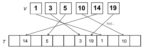
- map data (keys) to fixed-value sizes (values) using a
hash function to uniquely identify said data in a hash table
- in other words, convert keys into other values and store these new values at corresponding positions inside a table
- implemented using a dictionary (stores a set of elements where each element is identified via a unique key)
- universe U of keys with |U| = N (some very large positive integer)
- V \subseteq U: subset of actually used keys with |V| = n significantly smaller than N
- general idea: let T be an array with space for m elements (hash table) and a function h : U \to \{0, ..., m-1\} be used to map key to array index (hash function)
- probability of hash collisions for equally spread out hash positions: 1 - o(1)
// implementing a hash table with hash function
// only for dynamic dictionaries
void insert(Object e){
    T[h(key(e))] = e;
}

// only for dynamic dictionaries
void remove(Key k){
    T[h(k)] = null;
}

// for static and dynamic dictionaries
Object find(Key k){
    return T[h(k)];
}
// implementing a hash table with hash function
// only for dynamic dictionaries
void insert(Object e){
    T[h(key(e))] = e;
}

// only for dynamic dictionaries
void remove(Key k){
    T[h(k)] = null;
}

// for static and dynamic dictionaries
Object find(Key k){
    return T[h(k)];
}
Hashing with Chaining
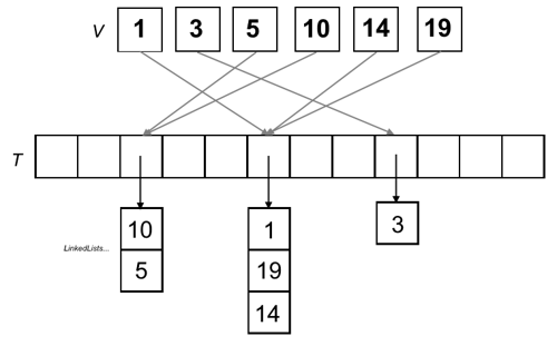
- idea: avoid collisions (different keys mapped to the same value) by having
each cell of the hash table point to a linked list containing the hashed values
- in other words, the hash table is an array, where each entry is a linked list
// init. array of linked lists
List<Object>[m] T;

// insert into linkedlist inside array
void insert(Object e){
    T[h(key(e))].insert(e);
}

// remove from linkedlist inside aray
void remove(Key k){
    T[h(k)].remove(k);
}

// find in linkedlist inside array
Object find(Key k){
    return T[h(k)].find(k);
}
// init. array of linked lists
List<Object>[m] T;

// insert into linkedlist inside array
void insert(Object e){
    T[h(key(e))].insert(e);
}

// remove from linkedlist inside aray
void remove(Key k){
    T[h(k)].remove(k);
}

// find in linkedlist inside array
Object find(Key k){
    return T[h(k)].find(k);
}- space complexity: O(n + m)
- time complexity:
insert(): O(1)remove(),find(): O(1 + n/m)- O(1 + c \cdot n/m) for c-universal hash families
Universal Hashing
- c > 0: constant
- H: family of hash functions
- m: size of hash, such that each hash function returns a hash code in range \{0,1,...,m-1\}
- a family of hash functions is c-universal,
if the probability of a hash collision between two keys x and y when
randomly chosing a hash function h \in
H is less
than or equal to \frac{c}{m}
- in other words: |\{h \in H : h(x) = h(y)\}| \leq \frac{c}{m}|H| for all x \neq y
- formally: \Pr[h(x) = h(y)] \leq \frac{c}{m} for all x \neq y
- (1-)universal family: c-universal family of
hash functions for c =
1
- in other words: |\{h \in H : h(x) = h(y)\}| \leq \frac{1}{m}|H| for all x \neq y
- formally: \Pr[h(x) = h(y)] \leq \frac{1}{m} for all x \neq y
- (*) how to determine, whether or not a given family is universal:
- statement: you are given a hash table of size m
(here m=4), a set of keys (*here
A,B,C,D,E)
and the given mappings for each hash function h_i
- example:
- h_1: A \mapsto 1, B \mapsto 1, C \mapsto 1, D \mapsto 3, E \mapsto 3
- h_2: A \mapsto 2, B \mapsto 2, C \mapsto 0, D \mapsto 0, E \mapsto 1
- h_3: A \mapsto 3, B \mapsto 1, C \mapsto 0, D \mapsto 3, E \mapsto 2
- h_4: A \mapsto 0, B \mapsto 2, C \mapsto 1, D \mapsto 2, E \mapsto 1
- h_5: A \mapsto 1, B \mapsto 3, C \mapsto 1, D \mapsto 2, E \mapsto 0
- h_6: A \mapsto 3, B \mapsto 2, C \mapsto 0, D \mapsto 1, E \mapsto 3
- example:
- question: is the hash family H_i (here H_1 = \{h_1, h_2, h_4, h_5\}) universal?
- answer: prove that |h \in H_1 : h(x) = h(y)| \leq 1
- step 1: note collisions between each possible pair for
each hash function
- A / B: h_1, h_2
- A / C: h_1, h_5
- A / D: \emptyset
- A / E: \emptyset
- B / C: h_1
- B / D: h_4
- B / E: \emptyset
- C / D: h_2
- C / E: h_4
- D / E: h_1
- step 2: check that the number of collisions at most 1 for
any given pair; if not, the function is not 1-universal, but
at least c
universal with c
being the number of collisions
- since |h \in H_1 : h(A) = h(B)| = |\{h_1, h_2\}| = 2, the family H_1 is c-universal for c \geq 2
- step 1: note collisions between each possible pair for
each hash function
- statement: you are given a hash table of size m
(here m=4), a set of keys (*here
A,B,C,D,E)
and the given mappings for each hash function h_i
- parameterized hash families: a hash function h_b = b \cdot x \mod m defines a family of
hash functions H =
\{h_b \; | \; b \in \Z\}
- b can be freely chosen, e.g. h_2 = 2x \mod m, h_{-400} = -400x \mod m
- if m is a prime number, then H = \{h_a : a \in \{0, ... , m-1\}^k \} with h_a(x) = a \cdot x \mod m is a universal family of hash functions
- lecture example - hashing an integer x:
- choose prime table size m
- e.g. m = 269
- let w = \lfloor \log_2
m\rfloor
- e.g. w = \lfloor \log_2 269\rfloor = 8
- separate bitstring x (binary
representation) into k
equal parts with w
bits each
- e.g. k = 4, since 4 \cdot 8 = 32
- interpret each part as an integer x_i \in [0, ..., 2^w-1]
- e.g. x_i \in [0, ..., 255] (an unsigned byte)
- interpret key x to compute
hash value of as k-vector
of x_i,
with x = (x_1, ..., x_k)^T, x_i
\in \{0, ..., 2^w-1\}
- e.g. x = (11, 7, 4, 3)^T
- define some vector a = (a_1, ..., a_k)^T, a_i \in \{0, ...,
m-1\}
- e.g. a = (2,4,261,16)^T
- scalar product of a and x is a \cdot x = \sum_{i = 1}^ka_ix_i
- define h_a : x \to \{0, ..., m-1\} as h_a(x) = a \cdot x \mod
m (scalar
product of a and
x,
product modulo m)
- e.g. h_a(x) = (2x_1 + 4x_2 + 261x_3 + 16x_4) \mod
269
- h_a(46915) = (2 \cdot 11 + 4 \cdot 7 + 261 \cdot 4 + 16 \cdot 3)\mod 269 = 66
- e.g. h_a(x) = (2x_1 + 4x_2 + 261x_3 + 16x_4) \mod
269
- choose prime table size m
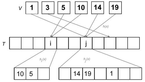
Perfect Hashing
- “remember: no collisions.”
- given:
- static dictionary S of length n with keys k_1, ..., k_n
- H_m: c-universal family of hash functions to \{0, ... m-1\}
- C(h): number of collisions in S for h for every pair (x,y)
- expected number of collisions: E[C(h)] \leq \frac{cn(n-1)}{m}
- for at least half of the functions, C(n) \leq 2cn(n-1)/m applies
- if m \geq cn(n-1)+1, then at least half of the functions h in H_m are injective (no collisions)
- strategy: double hashing with O(n) space complexity
- step 1: hash key using a well-chosen hash function in a table of size O(n) (i.e. m = \alpha n), where
each collision is packed into a bucket
- set \alpha to \sqrt 2 \cdot c, then m = \lceil \sqrt2 \cdot c \cdot n\rceil
- choose h with few collisions from H_{\lceil \sqrt2 \cdot c \cdot n\rceil} for h(k) \in \{0, ..., \lceil \sqrt2cn\rceil - 1\}
- choose h
until C(h) \leq \sqrt2 \cdot n
- formally: C(h) = |\{(x,y) \; | \; h(x) = h(y), x \neq y \}| \leq \sqrt2n
- note: every tuple pair is counted twice! (x,y), then (y,x)
- for each hash l,
a bucket B_l
is created, so that each key mapped to l
gets inserted into B_l
- each bucket has b_l = |B_l| keys
- each bucket has size m_l = c
\cdot b_l (b_l -1) + 1 \in O(b_l^2)
- sum of all bucket sizes effectively in O(n) due to low number of collisions
- (!) good function, when \alpha \mod x \implies x > \sqrt2 \cdot n for any \alpha
- step 2: choose fitting h_l
for bucket B_l
from c-universal
family H_{m_l}
with h_l(k) \in \{0, ..., m_l
-1\}
- choose h_l until no collisions
- (!) good function, when \alpha \mod x \implies x \geq b_l(b_l-1) + 1 for any \alpha with current bucket size b_l
- step 1: hash key using a well-chosen hash function in a table of size O(n) (i.e. m = \alpha n), where
each collision is packed into a bucket
- when using arrays, the hash value of a key x is s_l + h_l(x) with l = h(x), where h is a perfect hash function, and the worst-case runtime complexity for a lookup is O(1)
Linear Probing
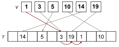
- open hash function, allowing for collision-causing entries to be inserted at a free neighbouring space
- idea: store element in next free space, scanning from left to right and
wrapping around
- the original hash value of a key is its ideal position
// insert into next available spot if ideal spot taken
void insert(Object e) {
    i = h(key(e));
    while (T[i] != null && T[i] != e)
        i = (i + 1) % m;
    T[i] = e;
}

// find object using linear search
Object find(Key k) {
    i = h(k);
    while (T[i] != null && key(T[i]) != k)
        i = (i+1) % m;
    return T[i];
}
// insert into next available spot if ideal spot taken
void insert(Object e) {
    i = h(key(e));
    while (T[i] != null && T[i] != e)
        i = (i + 1) % m;
    T[i] = e;
}

// find object using linear search
Object find(Key k) {
    i = h(k);
    while (T[i] != null && key(T[i]) != k)
        i = (i+1) % m;
    return T[i];
}- pros:
- no extra space complexity
- cache-efficient, since we only look at neighbouring entries in the same array
- deletion (move everything that is not on its ideal position
back one space until blank position reached, leave elements in ideal positions
where they are!):
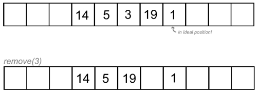
- runtime: O(1)
Sorting Algorithms and their Complexities
SelectionSort
- in-place, unstable, time complexity always \Theta(n^2), space complexity O(1)
- idea: choose smallest element from remainder of array and swap places with element at start of iteration
void selectionSort(Object[] a, int n) {
    for (int i = 0; i < n; i++) {
        int k = i;

        // find smallest element from unsorted sublist
        for (int j = i + 1; j < n; j++)
            if (a[j] < a[k])
                k = j;

        // swap with leftmost unsorted element
        swap(a, i, k);
    }
}
void selectionSort(Object[] a, int n) {
    for (int i = 0; i < n; i++) {
        int k = i;

        // find smallest element from unsorted sublist
        for (int j = i + 1; j < n; j++)
            if (a[j] < a[k])
                k = j;

        // swap with leftmost unsorted element
        swap(a, i, k);
    }
}- example:
| Sorted | Unsorted | Least (unsorted) |
|---|---|---|
| () | (11,25,12,22,64) | 11 |
| (11) | (25,12,22,64) | 12 |
| (11,12) | (25,22,64) | 22 |
| (11,12,22) | (25,64) | 25 |
| (11,12,22,25) | (64) | 64 |
| (11,12,22,25,64) | () |
InsertionSort
- in-place, stable, worst-case O(n^2), average-case O(n^2), best-case O(n), space complexity O(1)
- idea: take next element from array and insert into correct position by iterating backwards
void insertionSort(Object[] a, int n) {
    for (int i = 1; i < n; i++)
        // iterate backwards and insert at correct position
        for (int j = i − 1; j >= 0; j−−)
            if (a[j] > a[j + 1])
                swap(a, j, j + 1);
            else
                break;
}
void insertionSort(Object[] a, int n) {
    for (int i = 1; i < n; i++)
        // iterate backwards and insert at correct position
        for (int j = i − 1; j >= 0; j−−)
            if (a[j] > a[j + 1])
                swap(a, j, j + 1);
            else
                break;
}- example of a single iteration:
- array: [5,10,19,1,14,3]
- current element: 1
- [5,10,19,1,14,3] (correct position? no \to swap 1 and 19)
- [5,10,1,19,14,3] (correct position? no \to swap 1 and 10)
- [5,1,10,19,14,3] (correct position? no \to swap 1 and 10)
- [1,5,10,19,14,3] (correct position? yes)
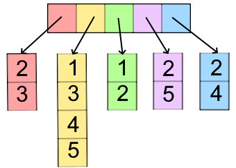
MergeSort
- not in-place, stable, worst-case O(n \log n), average-case \Theta(n \log n), best-case \Omega(n \log n), space complexity O(n)
- idea: split array recursively into two parts, then
merge together
- step 1: divide unsorted list recursively by halving it until each sublist only has one element
- step 2: merge until no sublists remain, with smaller elements coming before bigger ones in each step
- look, there’s a million different implementations of MergeSort, go find one that suits you best.
- example:
- divide:
- 10 , 5 , 7 , 19, 14 , 1 , 3
- 10 , 5 , 7 , 19 \;|\; 14 , 1 , 3
- 10 , 5 \;|\; 7 , 19 \;|\; 14 , 1 \;|\; 3
- 10 \;|\; 5 \;|\; 7 \;|\; 19 \;|\; 14 \;|\; 1 \;|\; 3
- conquer:
- 10 \;|\; 5 \;|\; 7 \;|\; 19 \;|\; 14 \;|\; 1 \;|\; 3
- 5,10 \;|\; 7 , 19 \;|\; 1,14 \;|\; 3
- 5,7,10,19 \;|\; 1,3,14
- 1,3,5,7,10,14,19
- divide:
QuickSort
- in-place, unstable, worst-case O(n^2), average-case O(n \log n), best-case O(n \log n), space complexity O(n)
- idea: choose pivot element, then split array into
elements smaller than pivot and greater or equal to pivot
- for each iteration, place pivot right at the end in the beginning for simplicity’s sake
- let
itemFromLeftbe the first element starting from the left of the array that is larger than the pivot anditemFromRightthe first element starting from the right of the array that is smaller than the pivot - once both have been found, swap places
- if the index of
itemFromLeft(i) is greater than that ofitemFromRight(j), stop and swap pivot withitemFromLeft's index - continue recursively for each array (lower or greater than pivot, leave pivot unchanged
in final array)
- speedup: when there are only two or less elements in an array, sort in one go without pivot element
void quickSort(int[] a, int l, int r) {
    if (l < r) {
        int p = a[r]; // choose rightmost element as pivot
        int i = l - 1; // left index
        int j = r; // right index
        do {
            // move left index
            do {
                i++;
            } while (a[i] < p);

            // move right index
            do {
                j--;
            } while (j >= l && a[j] > p);

            // swap elements if possible
            if (i < j)
                swap(a, i, j);
        } while (i < j);

        // at end of iteration, move pivot into correct position
        swap (a, i, r);
        // do quicksort for lower and greater subarrays
        quickSort(a, l, i - 1);
        quickSort(a, i + 1, r);
    }
}
void quickSort(int[] a, int l, int r) {
    if (l < r) {
        int p = a[r]; // choose rightmost element as pivot
        int i = l - 1; // left index
        int j = r; // right index
        do {
            // move left index
            do {
                i++;
            } while (a[i] < p);

            // move right index
            do {
                j--;
            } while (j >= l && a[j] > p);

            // swap elements if possible
            if (i < j)
                swap(a, i, j);
        } while (i < j);

        // at end of iteration, move pivot into correct position
        swap (a, i, r);
        // do quicksort for lower and greater subarrays
        quickSort(a, l, i - 1);
        quickSort(a, i + 1, r);
    }
}- example using rightmost element as pivot:
- current array: [10, 5, 19, 1, 14, 3]
- pivot: 3
- swapped 10 (first greater than 3 from left) and 1 (first smaller than 3 from right): [1, 5, 19, 10, 14, 3]
- new array: [1][3][19, 10, 14, 5]
- pivot: 5
- new array: [1][3][5][10, 14, 19]
- pivot: 19
- new array: [1][3][5][10, 14][19]
- pivot: 14
- final: [1][3][5][10][14][19]
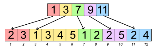
RadixSort
-
runtime always O(k \cdot n) with number of keys n and key length k, space complexity O(n + k)
-
idea: create and distribute elements into buckets according to their radix, then merge buckets and continue with new radix
- for decimal numbers: from rightmost digit to leftmost digit, create buckets for each present digit (0-9), distribute numbers into corresponding buckets, merge buckets and repeat for next digit of number
- for words: from rightmost letter to leftmost letter, create buckets for each present letter (A-Z), distribute words into corresponding buckets, merge buckets and repeat for next letter of word
-
example:
- array: 012, 203, 003, 074, 024, 017, 112
- buckets (rightmost digit): {012, 112}, {203, 003}, {074, 024}, {017}
- array: 012, 112, 203, 003, 074, 024, 017
- buckets (middle digit): {203, 003}, {012, 112, 017}, {024}, {074}
- array: 203, 003, 012, 112, 017, 024, 074
- buckets (leftmost digit): {003, 012, 017, 024, 074}, {112}, {203}
- final: 003, 012, 017, 024, 074, 112, 203
HeapSort
- in-place, unstable, runtime always O(n \log n), space complexity O(1)
- uses min-heap, sorts in reverse order (lowest to highest)
HeapSort(Object[] H, int n) {
    // build min-heap from array
    build(H[0], ... , H[n − 1]);
    // deleteMin until heap empty
    for (i = n − 1; i >= 1; i−−) {
        swap(H, 0, i);
        H.length−−;
        siftDown(H, 0);
    }
}
HeapSort(Object[] H, int n) {
    // build min-heap from array
    build(H[0], ... , H[n − 1]);
    // deleteMin until heap empty
    for (i = n − 1; i >= 1; i−−) {
        swap(H, 0, i);
        H.length−−;
        siftDown(H, 0);
    }
}- example[1]
Summary of Sorting Algorithm Complexities
| Algorithm | Best Case | Average Case | Worst Case | Space Complexity |
|---|---|---|---|---|
| SelectionSort | O(n^2) | O(n^2) | O(n^2) | O(1) |
| InsertionSort | O(n) | O(n^2) | O(n^2) | O(1) |
| MergeSort | O(n \log n) | O(n \log n) | O(n \log n) | O(n) |
| QuickSort | O(n \log n) | O(n \log n) | O(n^2) | O(n) |
| RadixSort | O(nk) | O(nk) | O(nk) | O(n + k) |
| HeapSort | O(n \log n) | O(n \log n) | O(n \log n) | O(1) |
Selection using QuickSelect
- idea: find k-th smallest
element in array of n elements
(numbering starts at 1)
- similar to QuickSort, but we only look at one partition of the array
- if k is smaller than the index of the pivot element (also starting at 1), continue with left array and same k
- if k is greater than the index of the pivot element, continue with right array and k = k - |a| - |b|, where |a| is the length of the left partition and |b| is the length of the middle partition (containing elements equal to pivot)
- else, element found
- example - finding 7th smallest element in array (5)
- s = [3,1,4,1,5,9,2,6,5,3,5,8,9], k = 7 \to [1,1][2][3,4,5,9,6,5,3,5,8,9]
- s = [3,4,5,9,6,5,3,5,8,9], k = 4 \to [3,4,5,5,3,5][6][9,8,9]
- s = [3,4,5,5,3,5], k = 4 \to [3,4,3][5,5,5][] \to found: 5
Recursion Analysis and Master Theorem
- divide-and-conquer algorithms: algorithms that recursively divide the problem into smaller subproblems, that are then solved (conquered) and merged back together
- runtime analysis of recursive functions is done using recurrence relations
- recurrence relations define one or more base cases and a function to determine the rest
- e.g. Fibonacci numbers F(x) = \begin{dcases}1 & \text{if n = 0}\\ 1 & \text{if n = 1} \\ F(n-2) + F(n-1) & \text{if n > 1}\end{dcases}
- to solve recurrence relation, we need to get rid of the function’s recursiveness and find a
closed form
- e.g. closed form of F(x) = \frac{1}{\sqrt 5}\left(\left(\frac{1 + \sqrt 5}{2}\right)^n - \left(\frac{1 - \sqrt 5}{2}\right)^n\right)
- method 1: iterative insertion
- write first few steps by hand and try to deduce closed formula
- e.g. T(n) = \begin{dcases}a
& \text{if n = 0} \\ T(n-1) + n & \text{if n > 0}
\end{dcases}
- T(1) = T(0) + 1 = a + 1
- T(2) = T(1) + 2 = a + 1 + 2
- T(3) = T(2) + 3 = a + 1 + 2 + 3
- generalized: T(n) = a + (1 + 2 + ... + n) = a + \frac{n(n+1)}{2} \in O(n^2)
- method 2: guess f(n) then prove by induction
- just wing it™
- e.g. T(n) = \begin{dcases}3
& \text{if n = 1} \\ T(n-1) + 2^n & \text{if n > 1}
\end{dcases}
- intuitively, guess that f(n) = 2^{n+1} - 1 and that T(n) \leq f(n) for n \geq 1
- in this case, we can prove that T(n) =
f(n)
- induction basis: for n = 1, T(1) = 3 = 2^{1+1} - 1
- induction hypothesis: T(n) = f(n) holds for some fixed n \in \N
- induction step: prove that T(n+1) = f(n+1)…
- as such, T(n) \in \Theta(f(n)), i.e. T(n) \in \Theta(2^n)
- method 3: master theorem
- follows a generalized formula of recurrence relations
- T(n) = \begin{dcases}a
& \text{if n = 1} \\ d \cdot T\left(\frac{n}{b}\right) + f(n) & \text{if n
>1}\end{dcases}
- a \in \Theta(1): runtime for base case (conquer)
- d: number of new subproblems per recursive layer
- b: factor, by which the size of new subproblems per recursive layer is reduced
- f(n) = c \cdot n \in \Theta(n): runtime needed by current layer for dividing and merging
- T(n) = \begin{dcases}\Theta(n) & \text{if d < b} \\ \Theta(n \log n) & \text{if d = b} \\ \Theta(n^{\log_bd}) & \text{if d > b} \end{dcases}
- example (mergesort):
- MergeSort splits the array in 2 (d) of size \frac{n}{2} \left(\frac{n}{b}\right) each for each recursive layer \to d = 2, b = 2
- the runtime of the base case is constant \to a \in \Theta(1)
- the runtime of dividing and merging for each layer is linear \to f(n) \in \Theta(n)
- T(n) = \begin{dcases}a & \text{if n = 1} \\ 2 \cdot T\left(\frac{n}{2}\right) + f(n) & \text{if n >1}\end{dcases}
- since d = b, then T(n) \in \Theta(n \log n)
Data Structures
Priority Queues
- abstract datatype, where each element is given a priority
| Operation | unsorted list | sorted list |
|---|---|---|
build() |
O(n) | O(n \log n) |
insert() |
O(1) | O(n) |
min() |
O(n) | O(1) |
deleteMin() |
O(n) | O(1) |
Binary Tree
- tree data structure, where each node (at most) has a left and a right
child (which themselves are binary trees)
- leaf: node without children
- inner node: node with at least one child
- depth t: number of edges from root to node (root depth 0)
- height h: depth from lowest node to root plus one (starting height 1)
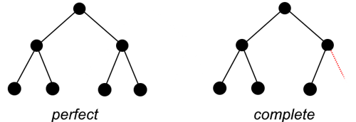
- perfect binary tree: 2^h-1 nodes, 2^{h-1}
leaves
- a full binary tree with n nodes has height \lfloor \log_2(n) \rfloor + 1
- complete binary tree: the first t-1 levels make up a
complete binary tree, there exists a node e on level
t such that
there are no more nodes to the right of it
- modifying a binary tree:
insert(): O(\log n)
delete(): O(\log n)
Binary Heaps
- binary tree with…
- form invariant: all layers are complete except for lowest layer
- heap invariant (min-heap): \text{key(v.parent)} \leq \text{key(v)}
- can be stored using arrays, where a node with index i has children at
indices 2i + 1 and 2i + 2 and parent node at \lfloor \frac{i-1}{2}
\rfloor
deleteMin(): replace root with last element in heap and sift down until heap invariant fulfilled, \mathcal{O}(1) + runtime ofsiftDown(v)
// pseudocode
Element deleteMin(Heap<Element> H) {
    Element min = root of H;
    replace root of H with last element of H;
    siftDown(H, root of H);
    return min;
}
// pseudocode
Element deleteMin(Heap<Element> H) {
    Element min = root of H;
    replace root of H with last element of H;
    siftDown(H, root of H);
    return min;
}siftDown(v): move node down according to min-heap invariant, \mathcal{O}(\log n)
// pseudocode
siftDown(Heap<Element> H, Node v) {
    // cannot sift down if node is leaf
    if (isLeaf(v)) return;

    Node m;
    // choose direction
    if (key(v.left) < key(v.right)){
        m = v.left;
    }
    else {
        m = v.right;
    }

    // restore heap invariant or quit
    if (key(m) < key(v)) {
        swap content of m and v;
        siftDown(H, m);
    }
}
// pseudocode
siftDown(Heap<Element> H, Node v) {
    // cannot sift down if node is leaf
    if (isLeaf(v)) return;

    Node m;
    // choose direction
    if (key(v.left) < key(v.right)){
        m = v.left;
    }
    else {
        m = v.right;
    }

    // restore heap invariant or quit
    if (key(m) < key(v)) {
        swap content of m and v;
        siftDown(H, m);
    }
}insert(e): insert element at end of heap then sift up into place, \mathcal{O}(1) + runtime ofsiftUp()
// pseudocode
insert(Heap<Element> H, Element e) {
    Node v = insert e at end of H;
    siftUp(H, v);
}
// pseudocode
insert(Heap<Element> H, Element e) {
    Node v = insert e at end of H;
    siftUp(H, v);
}siftUp(v): move node up according to min-heap invariant, \mathcal{O}(\log n)
// pseudocode
siftUp(Heap<Element> H, Node v) {
    while (v is not root && key(v.parent) > key(v)) {
        swap content of v and v.parent;
        v = v.parent;
    }
}
// pseudocode
siftUp(Heap<Element> H, Node v) {
    while (v is not root && key(v.parent) > key(v)) {
        swap content of v and v.parent;
        v = v.parent;
    }
}build(e1...en):- insert n elements unsorted into heap
- do
siftDown()for each node v on layer t bottom-up in reverse order (right to left)- in other words: the first \lfloor n / 2
\rfloor elements of
the actual array, handled in reverse order (e.g. for
[15,20,9,1,11,8,4,13,17], one would dosiftDown()for1,9,20,15in that order)
- in other words: the first \lfloor n / 2
\rfloor elements of
the actual array, handled in reverse order (e.g. for
decreaseKey(v,k): \mathcal{O}(\log n)
decreaseKey(Heap<Element> H, Node v, int k) {
    if (k > key(v)) error();
    key(v) = k;
    siftUp(H, v);
}
decreaseKey(Heap<Element> H, Node v, int k) {
    if (k > key(v)) error();
    key(v) = k;
    siftUp(H, v);
}increaseKey(v,k): \mathcal{O}(\log n)
increaseKey(Heap<Element> H, Node v, int k) {
    if (k < key(v)) error();
    key(v) = k;
    siftDown(H, v);
}
increaseKey(Heap<Element> H, Node v, int k) {
    if (k < key(v)) error();
    key(v) = k;
    siftDown(H, v);
}delete(v): replace v with last node v' in heap then dosiftUp(v')orsiftDown(v')
Binary Heap example using Max-Heap
- insertion: adding 15 into heap by inserting it at the end, then sifting up until heap
invariant (here max-heap, i.e. \text{key(parent) > key(child)})
is restored
- for visualization: let X be the spot where 15 will be inserted at first

- place 15 there and check, if heap invariant is maintained \to since heap invariant
is violated, sift 15 up and check again

- since the heap invariant is violated once more, sift up once again \to since the node is now
at the root, we have successfully inserted the node into the heap

- for visualization: let X be the spot where 15 will be inserted at first
- deletion: using the same max-heap as before
- let 11 be the node we want to remove (equiv.
deleteMax())
- replace 11 with last node in heap, 4

- sift down, then heap invariant is restored

- let 11 be the node we want to remove (equiv.
Binomial Trees
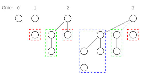
- a binomial tree of rank r has a root
node with children of rank r-1, r-2, … , 0 in that order[2]
- maximum depth r
- depth l \in \{0, ... ,r\} has r \choose l nodes (\frac{r!}{l!(r-l)!})
- in total 2^r nodes
- maximum degree r in root
- merging: root node with bigger key becomes new child of root with smaller key[3]
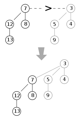
- removing root: new binomial trees of ranks r-1 down to 0 appear
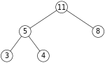
Binomial Heaps
-
set of binomial trees where each tree fulfills the min-heap invariant, there are no two trees with the same rank and a min-pointer points to the root with the smallest key
-
a binomial heap with n nodes contains at most 1 + \lfloor \log_2(n) \rfloor binomial trees
- the binary representation of n tells us
exactly the rank of the trees in our heap
- z.B. n = 11_{10} = 1011_b = 1 * 2^3 + 1 * 2^1 + 1 * 2^0 \to there are trees of ranks 3,1,0
- the binary representation of n tells us
exactly the rank of the trees in our heap
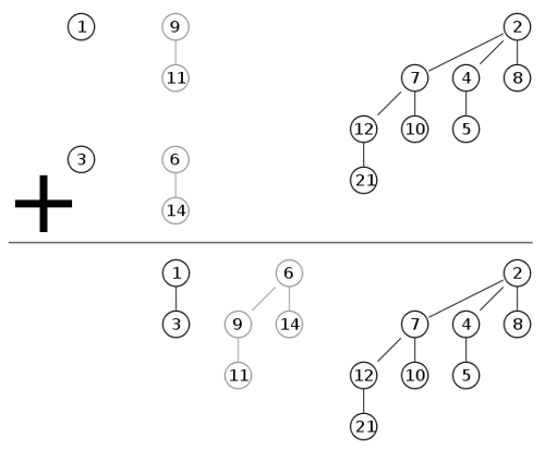
-
merging: equivalent to binary addition, \mathcal{O}(\log n) with n = \max\{n_1,n_2\}[4]
-
operations:
min(): return root with minimal key (located at min-pointer)- \mathcal{O}(1)
merge(): equivalent to binary addition- \mathcal{O}(\log n)
insert(e):merge()with binomial tree of rank 0, containing onlye- \mathcal{O}(\log n)
deleteMin(): remove min-root andmerge()the children with the rest of the heap- \mathcal{O}(\log n)
decreaseKey(v,k): setkey(v) = k, thensiftUp()in binomial tree ofvand adjust min-pointer if needed- \mathcal{O}(\log n)
remove(v): firstdecreaseKey(v, -inf), thendeleteMin()- \mathcal{O}(\log n)
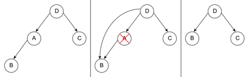
Binary Search Tree

- binary tree with…
- search tree invariant: left child smaller than parent, right child larger than parent
- key invariant: each key is unique
- degree invariant: a node can only have at most 2 children
locate(e): begin at root w of tree, O(\log n)- if \text{key}(v) \geq k, go to left child, else go to right child
- return minimal node for which its key is greater or equal e
insert(e): O(\log n)- do
locate(key(e))until e' is reached - if \text{key}(e') > \text{key}(e), insert e before e' in list, and create new search tree node with \text{key}(e) as splitter key to fulfill search tree invariant
- else, throw error
- do
remove(k): O(\log n)- do
locate(k)until e is reached - if \text{key}(e) =
k
- delete e from list
- delete parent key v from tree
- if not already deleted, replace node with next smaller node in tree
- else, throw error
- do
- cba with making original graphics here, just look in the slides or google it, the examples are good enough
AVL-Trees
- self-balancing binary search trees
- fixes and height-balancing possibly needed after insertion and deletion
- for any node, the height of its two subtrees differs by at most 1
- balance factor = height of right subtree - height of left subtree \in \{-1,0,1\}[5]
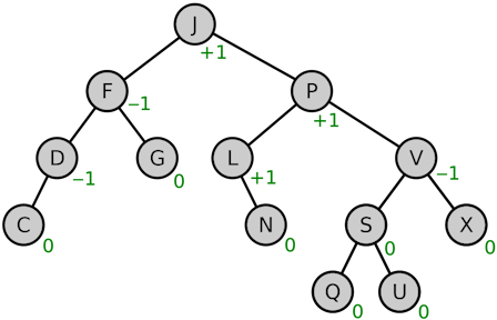
- balance factor = height of right subtree - height of left subtree \in \{-1,0,1\}[5]
- time complexity: worst-case O(\log n), best-case \Theta(\log n)
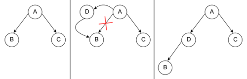
- inserting: start
at root; if k_{current} \geq v, go left,
otherwise right; insert where free space available then rotate
- left rotation if balance factor of node is 2 and balance factor of right child is +1 or 0
- right rotation if balance factor of node is -2 and balance factor of left child is -1 or 0
- right-left rotation if balance factor of node is +2 and right child has balance factor -1
- left-right rotation if balance factor of node is -2 and left child has balance factor of +1
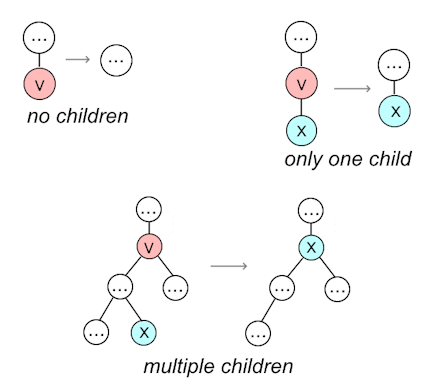
- deleting:
- if node does not have a left child, move right child into its place
- if node does not have a right child, move left child into its place
- if node has left and right child, replace with node with next
smaller key
- balancing afterwards: same as before
- searching works the same as in any standard binary search tree
Summary: AVL-Tree Rotations
- if height differences for parent and child have the same sign,
perform single rotation
- if positive, perform left rotation
- if negative, perform right rotation
- if height differences for parent and child have different signs,
perform double rotation
- if +2 / -1, perform R-L–rotation
- if -2 / +1, perform L-R-rotation
Source: https://www.geeksforgeeks.org/insertion-in-an-avl-tree/
T1, T2, T3 and T4 are subtrees.
S - single, D - double

S: RIGHT ROTATE
         z                                      y
        / \                                   /   \
       y   T4      Right Rotate (z)          x      z
      / \          - - - - - - - - ->      /  \    /  \
     x   T3                               T1  T2  T3  T4
    / \
  T1   T2

D: LEFT-RIGHT ROTATE
     z                               z                           x
    / \                            /   \                        /  \
   y   T4  Left Rotate (y)        x    T4  Right Rotate(z)    y      z
  / \      - - - - - - - - ->    /  \      - - - - - - - ->  / \    / \
T1   x                          y    T3                    T1  T2 T3  T4
    / \                        / \
  T2   T3                    T1   T2

S: LEFT ROTATE
  z                                y
 /  \                            /   \
T1   y     Left Rotate(z)       z      x
    /  \   - - - - - - - ->    / \    / \
   T2   x                     T1  T2 T3  T4
       / \
     T3  T4

D: RIGHT-LEFT ROTATE
   z                            z                            x
  / \                          / \                          /  \
T1   y   Right Rotate (y)    T1   x      Left Rotate(z)   z      y
    / \  - - - - - - - - ->     /  \   - - - - - - - ->  / \    / \
   x   T4                      T2   y                  T1  T2  T3  T4
  / \                              /  \
T2   T3                          T3   T4
(a,b)-Trees
- variable definitions:
- w: root
- n leaves
- d(v): number of children (ext. degree) of a node v
- t(v): depth of a node v
- a search tree G is called an (a,b)-tree for a \geq 2 and b \geq 2a-1 (alt. a \leq \frac{b+1}{2}) if
following invariants are fulfilled:
- form invariant: all leaves are at the same depth
- degree invariant: for all internal nodes except for the root, a \leq d(v) \leq
b
- in other words, each node (except for the root) has at least a and at most b children
- for the root node: 2 \leq d(w) \leq b (except if it’s a leaf)
- depth d \leq 1 + \lfloor \log_a \frac{n+1}{2}\rfloor if n > 1
- all operations \Theta(\log n)
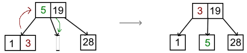
locate(k)works the same as in any search treeinsert(e):- locate e'
using
locate(key(e)) - if \text{key}(e) < \text{key}(e'), insert e before e', otherwise throw error
- insert \text{key}(e) and handle in v
into tree
- case 1: if d(v) \leq b, finish
- case 2: if d(v) > b, split v in two and move splitter key (usually key at index \lfloor b / 2 \rfloor or median) up
- case 2.5: if degree of parent node is now bigger, continue until eventually \deg \leq b or root has been split
- locate e'
using
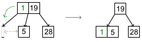
remove(e):- let v be
the node of e
- case 1: v
contains e
(lowest depth)
- directly delete e and v
- if v now has less than a children, steal or merge
- case 2: v
does not contain e
(not on lowest depth)
- let e' be the element directly before e, included in v
- delete e' from v and e from list
- replace remaining e in tree with e' (i.e. replace key with value which contained pointer to e)
- if v now has less than a children, steal or merge
- case 1: v
contains e
(lowest depth)
- steal if neighbouring node v'
of v
has more than a children,
start with left neighbour
- v' left of v: rightmost key in v' goes up, replaced key goes down into v
- v'
right of v:
leftmost key in v'
goes up, replaced key goes down into v
- merge if neighbouring node v'
of v
does not have more than a children
- merge v with neighbouring node, preferably left node, by bringing down father element
- father node and adjacent nodes may need to be adjusted with steal / merge too afterwards, since we’re taking a node away from it
- if root is empty, remove it
- let v be
the node of e
- for the same reason as before, if you want examples, look in the slides and go along with those
Graphs
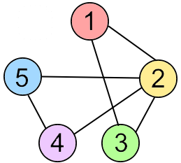
- representing a graph:
- list of edges
- \{1,2\}, \{1,3\}, \{2,3\}, \{2,4\}, \{2,5\}, \{4,5\}
- +: O(m) space
complexity,
insert(Edge e),insert(Node v)andremove(Key i)in O(1) - -:
find(Key i, Key j)andremove(Key i, Key j)worst-case \Theta(m)
- adjacency matrix
- \begin{pmatrix}0&1&1&0&0\\1&0&1&1&1\\1&1&0&0&0\\0&1&0&0&1\\0&1&0&1&0\end{pmatrix}
- +: can tell in O(1) if two nodes are neighbors, inserting and deleting edges in O(1)
- -: space complexity \Theta(n^2), finding all neighbors of a node costs O(n) time
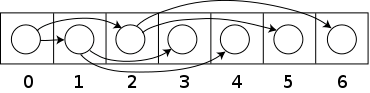
- adjacency arrays (top: indices of node in bottom array, bottom:
neighboring node keys)
- +: space complexity n + m + \Theta(1) for directed graphs and n + 2m + \Theta(1) for undirected graphs
- -: inserting and deleting edges is costly
- adjacency lists (similar to arrays, but with linked lists)
- +: inserting edges in O(1), deleting
edges in O(d) or O(1) with handle
- when using adjacency lists with a hash table, all operations can be done in O(1)
- -: usage of lists requires heap space and generally takes longer
- when using adjacency lists with a hash table, the space complexity becomes O(n + m)
- +: inserting edges in O(1), deleting
edges in O(d) or O(1) with handle
- list of edges
- traversing a graph (O(|V|
+ |E|)):
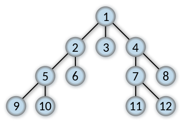
- breadth-first-search
- horizontal before vertical
- operates based on a FIFO-queue
- useful for SSSP (single source shortest path) due to storing distance of each node to source
- algorithm:
- insert node in queue
- take front item of queue and add it to visited list
- create list of vertex’s adjacent nodes, add ones not yet visited to the back of the queue
- repeat steps 2 and 3 until queue is empty
- order of expansion[6]:
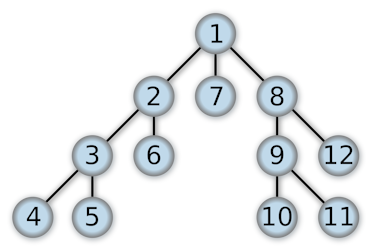
- depth-first search
- vertical before horizontal
- operates based on a stack
- algorithm:
- insert node onto stack
- take top item of stack and add it to visited list
- create list of vertex’s adjacent nodes, add ones not yet visited to the top of the stack
- repeat steps 2 and 3 until stack is empty
- order of expansion[7]:
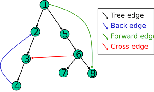
- extra variables:
dfsNum: exploration orderfinishNum: finished order
- types of edges:
- root edge: edge from root outwards
- forwards edge: to a successor
- backwards edge: to a predecessor
- breadth-first-search
- using DFS to recognize DAGs:
- DFS does not contain any backwards edges
- for all edges (v,w),
finishNum[v] > finishNum[w](higher finish number points to lower finish number)
| Type of Edge | dfsNum[v] < dfsNum[w] |
finishNum[v] > finishNum[w] |
|---|---|---|
| Root Edge | yes | yes |
| Forwards Edge | yes | yes |
| Backwards Edge | no | no |
| Rest | no | yes |
Connectivity
-
a graph is connected if every pair of vertices in the graph is connected \equiv there is a path between every pair of vertices
-
a graph with just one vertex is connected
- an edgeless graph with two or more vertices is disconnected
-
a directed graph is called weakly connected if replacing all of its directed edges with undirected edges produces a connected (undirected) graph
-
it is unilaterally connected if it contains a directed path from u to v or a directed path from v to u for every pair of vertices u, v
-
it is strongly connected, or simply strong, if it contains a directed path from u to v and a directed path from v to u for every pair of vertices u, v
-
a connected component is a maximal connected subgraph of an undirected graph
- each vertex belongs to exactly one connected component, as does each edge
- a graph is connected if and only if it has exactly one connected component
-
the strong components are the maximal strongly connected subgraphs of a directed graph
Shortest Paths (SSSP)
- case 1: edge costs 1 \to BFS
- case 2: DAG, variable edge costs \to Topological Sorting
- case 3: variable graph, positive edge costs \to Dijkstra
- case 4: variable graph, variable edge costs \to Bellman-Ford
DAG - Topological Sorting
L ← Empty list that will contain the sorted elements
S ← FIFO-Queue of all nodes with no incoming edge

while S is not empty do
    remove a node n from S
    add n to L
    for each node m with an edge e from n to m do
        remove edge e from the graph
        if m has no other incoming edges then
            insert m into S

if graph has edges then
    return error   (graph has at least one cycle)
else
    return L   (a topologically sorted order)
Dijkstra’s Algorithm
- used to find shortest paths between nodes in a weighted graph with positive weights
- algorithm:
- mark all nodes unvisited and create set of unvisited nodes
- assign tentative distances to each node (0 for initial node, \infty for all other nodes)
- the tentative distance of a node is the length of the shortest path (so far) between said node and the starting node
- for the current node, calculate tentative distances of neighboring unvisited nodes
through current node
- if newly calculated tentative distance is smaller than current distance, replace current distance with tentative distance
- mark current node as visited (remove from unvisited set)
- if destination node is marked as visited or if smallest tentative distance among nodes in unvisited set is infinity, stop
- else, go to unvisited node with smallest tentative distance and go back to third step
- time complexity: O(|E| + |V| \log |V|)
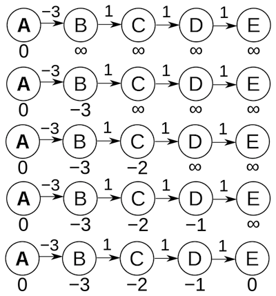
Bellman-Ford[8]
- works on graphs with negative edge weights
- fundamental idea: there are at most |V| - 1 edges in one of our paths (because if there were |V| or more, there would be a cycle)
- algorithm:
- initialize distance to source to 0 and all other nodes to infinity
- for all edges: if the distance to the destination can be shortened by taking the
edge, the distance is updated to the new lower value
- if dist[v] > dist[u] + weight((u,v)), then dist[v] = dist[u] + weight((u,v))
- repeat last step |V|-1 times
- if in the last iteration, distances are still being updated, then finally
update these distances to - \infty, indicating
that there is a negative weight cycle
- if in the last iteration, distances are still being updated, then finally
update these distances to - \infty, indicating
that there is a negative weight cycle
- time complexity: O(|E| \cdot |V|)
Shortest Paths (APSP)
Floyd-Warshall’s Algorithm
- O(n^3), please don’t use this
let dist be a |V| × |V| array of minimum distances initialized to ∞ (infinity)
for each edge (u, v) do
    dist[u][v] ← w(u, v)
for each vertex v do
    dist[v][v] ← 0
for k from 1 to |V|
    for i from 1 to |V|
        for j from 1 to |V|
            if dist[i][j] > dist[i][k] + dist[k][j]
                dist[i][j] ← dist[i][k] + dist[k][j]
            end if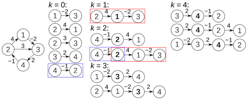
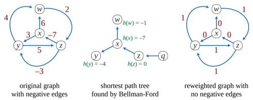
Johnson’s Algorithm
- insert new temporary node s with edge (s,v) to all v and c(s,v) = 0
- calculate d[s,v] using Bellman-Ford’s Algorithm and set \phi[v] = d[s,v] for all v
- calculate modified edge costs \overline c(e) = \phi(v) + c(e) - \phi(w)
- calculate \overline d[v,w] for all v without s using Dijkstra’s Algorithm using the modified costs
- calculate proper distances d[v,w] = \overline d[v, w] + \phi [w] - \phi [v]
- example: first 3 stages
Minimum Spanning Trees
- Kruskal’s
Algorithm (O(m
\log m)):
- repeatedly choose a minimum-cost edge connecting two connected components until only
one connected component remains[9]
- repeatedly choose a minimum-cost edge connecting two connected components until only
one connected component remains[9]
- Prim’s
Algorithm:
- look at growing tree T, initially consisting of any single node s
- add to T an edge with minimal weight from a tree node to a node outside the tree (if there are multiple possibilities, it doesn’t matter which)
- repeat selection until all n nodes in
tree[10]
-
source: “https://commons.wikimedia.org/wiki/File:Heapsort-example.gif”, Swfung8 on Wikimedia, 19.04.2011, licensed under CC BY-SA 3.0, no changes made ↩︎
-
source: “https://en.wikipedia.org/wiki/File:Binomial_Trees.svg”, Lemontea (?) on Wikipedia, 19.03.2006, licensed under CC BY-SA 3.0, no changes made ↩︎
-
source: https://en.wikipedia.org/wiki/File:Binomial_heap_merge1.svg, Lemontea on Wikipedia, 15.05.2006, licensed under CC BY-SA 3.0, no changes made ↩︎
-
source: https://en.wikipedia.org/wiki/File:Binomial_heap_merge2.svg, Lemontea on Wikipedia, 15.05.2006, licensed under CC BY-SA 3.0, no changes made ↩︎
-
source: https://en.wikipedia.org/wiki/File:AVL-tree-wBalance_K.svg, Nomen4Omen on Wikipedia, 01.06.2016, licensed under CC BY-SA 4.0, no changes made ↩︎
-
source: https://en.wikipedia.org/wiki/File:Breadth-first-tree.svg, Alexander Drichel on Wikipedia, 28.03.2008, licensed under CC BY 3.0, no changes made ↩︎
-
source: https://commons.wikimedia.org/wiki/File:Depth-first-tree.svg, Alexander Drichel on Wikimedia, 28.03.2008, licensed under CC BY 3.0, no changes made ↩︎
-
source: https://commons.wikimedia.org/wiki/File:Bellman–Ford_algorithm_example.gif, Michel Bakni, Thomas H. Cormen, Charles E. Leiserson, Ronald L. Rivest, Clifford Stein (2001) Introduction to Algorithms (2nd ed.), p. 589 ISBN: 9780262032933, 01.05.2021, licensed under CC BY-SA 4.0, no changes made ↩︎
-
source: https://en.wikipedia.org/wiki/File:KruskalDemo.gif, Shiyu Ji on Wikipedia, 24.12.2016, licensed under CC BY-SA 4.0, no changes made ↩︎
-
source: https://en.wikipedia.org/wiki/File:PrimAlgDemo.gif, Shiyu Ji on Wikipedia, 24.12.2016, licensed under CC BY-SA 4.0, no changes made ↩︎